If you assign quasi-stellar objects (QSOs) to incremental apparent magnitude bins, arranged in a bright-to-dim sequence, then produce redshift histograms for the bins, you might expect to see a set of broad low-amplitude skewed bell-shaped curves whose maxima systematically slide toward higher redshifts for dimmer and dimmer apparent magnitudes. The set of adjoining histograms, thus produced, would be a kind of redshift "CAT scan."

To see if the above idea is borne out by published data (or not), objects listed in the CD-ROM version of the 1993 Hewitt & Burbidge QSO Catalog(1) were analyzed using a computer program called Z-Mag-B. The program assigned QSOs to redshift-apparent magnitude bins. One set of bins was for North Galactic QSOs and the other set was for South Galactic QSOs.

Z-Mag-B selected 6574 objects from the QSO catalog. This number includes 165 unique low-redshift objects that are mostly called active galactic nuclei (AGNs). These are characterized by the H I (4861) - O III (4959, 5007) triplet. (Objects whose whose magnitudes had been rounded off to the nearest integer, were not used.)

QSOs used in this analysis are as follows:

The figures for the AGNs, et.al., (which are included, above) are:

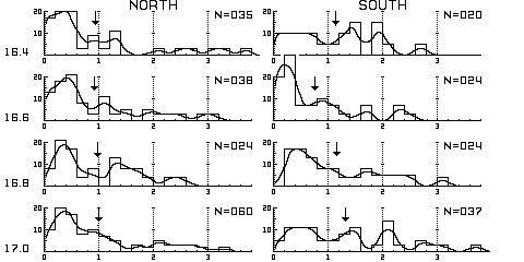
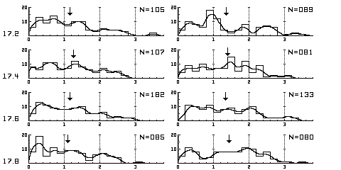
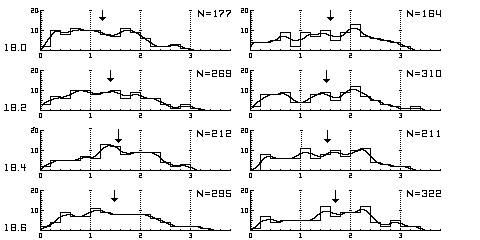
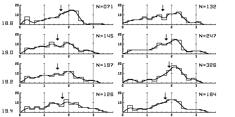
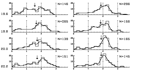
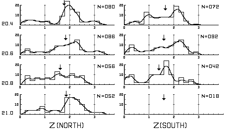
Once the redshift-apparent magnitude bins were filled, they were segregated into magnitude limited samples. Each sample has an apparent magnitude thickness of 0.2. The magnitude values shown with each histogram correspond to the brighter edge of the sample.

The overall QSO redshift-magnitude diagrams (not shown in this web page) turn out to not be statistically "normal" nor are the individual magnitude-limited redshift histograms produced in this study. Many of the latter appear to contain a broad (redshift-wise) continuum and often one fairly well defined peak (sometimes two). No statement is made, at present, about the statistical significance or insignificance of the differences between paired North-South samples. In a planned update to this page, Kolomogorov-Smirnov tests will be applied to them to quantify their differences.

Before getting to the redshift histograms, the following diagram is shown to depict the redshift averages for the sequential magnitude bins for North and South galactic QSOs. It can be seen, that for the brighter samples, the averages constitute more than a scatter diagram. They increase in average redshift with decreasing apparent magnitude. In general, the Southern samples are more redshifted than the Northern samples. [Arp cautions that search mode bias, for example, radio vs optical, may be a factor in the net redshift differences between the galactic hemispheres.(2)] There is a relative redshift inversion at magnitude v = 20.3, i.e., the Northern galactic QSOs become more redshifted than the Southern QSOs. Both groups also appear to level off in redshift with further decreases in magnitude. If these effects are more than statistical fluctuations or search bias artifacts, they will be important with regard to our overall understanding of QSOs. [There is a reported shortage of detected very high redshift QSOs at faint apparent magnitudes(3).]

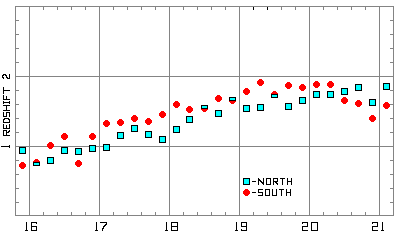
QSO Redshift Averages for Apparent Magnitude Bins

Normalized redshift histograms for each apparent magnitude limited sample were then produced. The normalization process reduces search mode bias and facilitates comparisons between samples. The plots below are the normalized redshift histograms for the magnitude limited samples in the range v = 16.4 to 21.0. Northern galactic QSO histograms are on the left and those for Southern galactic QSOs are on the right. [Histograms shown are based on sample sizes (raw data) having at least 20 objects in them.]

Natural smoothing, where added, is based on the following relations.

Smoothed values for the junctions between adjacent bins are equal to their arithmetic means. The curves which connect the smoothed points are hand drawn.

The y-axis for each histogram is "Normalized Number per delta v = 0.2."
The x-axis for each histogram is Redshift.
Downward pointing arrows, where shown, represent the average redshift for the sample.